In previous posts, I used popular machine learning algorithms to fit models to best predict MPG using the cars_19 dataset which is a dataset I created from publicly available data from the Environmental Protection Agency. It was discovered that support vector machine was clearly the winner in predicting MPG and SVM produces models with the lowest RMSE. In this post I am going to use LightGBM to build a predictive model and compare the RMSE to the other models.
The raw data is located on the EPA government site.
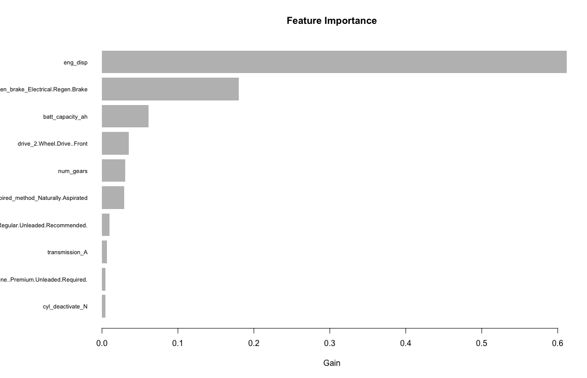
Similar to the other models, the variables/features I am using are: Engine displacement (size), number of cylinders, transmission type, number of gears, air inspired method, regenerative braking type, battery capacity Ah, drivetrain, fuel type, cylinder deactivate, and variable valve. The LightGBM package does not handle factors so I will have to transform them into dummy variables. After creating the dummy variables, I will be using 33 input variables.
str(cars_19)
'data.frame':    1253 obs. of  12 variables:
 $ fuel_economy_combined: int  21 28 21 26 28 11 15 18 17 15 ...
 $ eng_disp             : num  3.5 1.8 4 2 2 8 6.2 6.2 6.2 6.2 ...
 $ num_cyl              : int  6 4 8 4 4 16 8 8 8 8 ...
 $ transmission         : Factor w/ 7 levels "A","AM","AMS",..: 3 2 6 3 6 3 6 6 6 5 ...
 $ num_gears            : int  9 6 8 7 8 7 8 8 8 7 ...
 $ air_aspired_method   : Factor w/ 5 levels "Naturally Aspirated",..: 4 4 4 4 4 4 3 1 3 3 ...
 $ regen_brake          : Factor w/ 3 levels "","Electrical Regen Brake",..: 2 1 1 1 1 1 1 1 1 1 ...
 $ batt_capacity_ah     : num  4.25 0 0 0 0 0 0 0 0 0 ...
 $ drive                : Factor w/ 5 levels "2-Wheel Drive, Front",..: 4 2 2 4 2 4 2 2 2 2 ...
 $ fuel_type            : Factor w/ 5 levels "Diesel, ultra low sulfur (15 ppm, maximum)",..: 4 3 3 5 3 4 4 4 4 4 ...
 $ cyl_deactivate       : Factor w/ 2 levels "N","Y": 1 1 1 1 1 2 1 2 2 1 ...
 $ variable_valve       : Factor w/ 2 levels "N","Y": 2 2 2 2 2 2 2 2 2 2 ...
One of the biggest challenges with this dataset is it is small to be running machine learning models on. The train data set is 939 rows and the test data set is only 314 rows. In an ideal situation there would be more data, but this is real data and all data that is available.
After getting a working model and performing trial and error exploratory analysis to estimate the hyperparameters, I am going to run a grid search using:
max_depth

num_leaves

num_iterations

early_stopping_rounds

learning_rate
As a general rule of thumb num_leaves = 2^(max_depth) and num leaves and max_depth need to be tuned together to prevent overfitting. Solving for max_depth:
max_depth = round(log(num_leaves) / log(2),0)This is just a guideline, I found values for both hyperparameters higher than the final hyper_grid below caused the model to overfit.
After running a few grid searches, the final hyper_grid I am looking to optimize (minimize RMSE) is 4950 rows. This runs fairly quickly on a Mac mini with the M1 processor and 16 GB RAM making use of the early_stopping_rounds parameter.
#grid search
#create hyperparameter grid
num_leaves =seq(20,28,1)
max_depth = round(log(num_leaves) / log(2),0)
num_iterations = seq(200,400,50)
early_stopping_rounds = round(num_iterations * .1,0)

hyper_grid <- expand.grid(max_depth = max_depth,
                          num_leaves =num_leaves,
                          num_iterations = num_iterations,
                          early_stopping_rounds=early_stopping_rounds,
                          learning_rate = seq(.45, .50, .005))

hyper_grid <- unique(hyper_grid)for (j in 1:nrow(hyper_grid)) {
set.seed(123)
light_gbn_tuned <- lgb.train(
params = list(
objective = "regression",
metric = "l2",
max_depth = hyper_grid$max_depth[j],
num_leaves =hyper_grid$num_leaves[j],
num_iterations = hyper_grid$num_iterations[j],
early_stopping_rounds=hyper_grid$early_stopping_rounds[j],
learning_rate = hyper_grid$learning_rate[j]
#feature_fraction = .9
),
valids = list(test = test_lgb),
data = train_lgb
)
yhat_fit_tuned <- predict(light_gbn_tuned,train[,2:34])
yhat_predict_tuned <- predict(light_gbn_tuned,test[,2:34])
rmse_fit[j] <- RMSE(y_train,yhat_fit_tuned)
rmse_predict[j] <- RMSE(y_test,yhat_predict_tuned)
cat(j, "\n")
}
set.seed(123)
light_gbn_final <- lgb.train(
  params = list(
    objective = "regression",
    metric = "l2",
    max_depth = 4,
    num_leaves =23,
    num_iterations = 400,
    early_stopping_rounds=40,
    learning_rate = .48
    #feature_fraction = .8
  ),
  valids = list(test = test_lgb),
  data = train_lgb
)
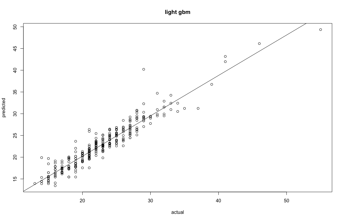
postResample(y_test,yhat_predict_final)
     RMSE  Rsquared       MAE
1.7031942 0.9016161 1.2326575
sum(abs(r) <= rmse_predict_final) / length(y_test)  #[1] 0.7547771
[1] 0.7547771
> sum(abs(r) <= 2 * rmse_predict_final) / length(y_test) #[1] 0.9522293
[1] 0.9522293
>
> summary(r)
     Min.   1st Qu.    Median      Mean   3rd Qu.      Max.
-11.21159  -0.96398   0.06337  -0.02708   0.96796   5.77861
Comparison of RMSE:

svm = .93
lightGBM = 1.7
XGBoost = 1.74
gradient boosting = 1.8
random forest = 1.9
neural network = 2.06
decision tree = 2.49
mlr = 2.6