In the previous four posts I have used multiple linear regression, decision trees, random forest, gradient boosting, and support vector machine to predict MPG for 2019 vehicles. It was determined that
svm produced the best model. In this post I am going to use the
neuralnet package to fit a neural network to the cars_19 dataset.
The raw data is located on the
EPA government site.
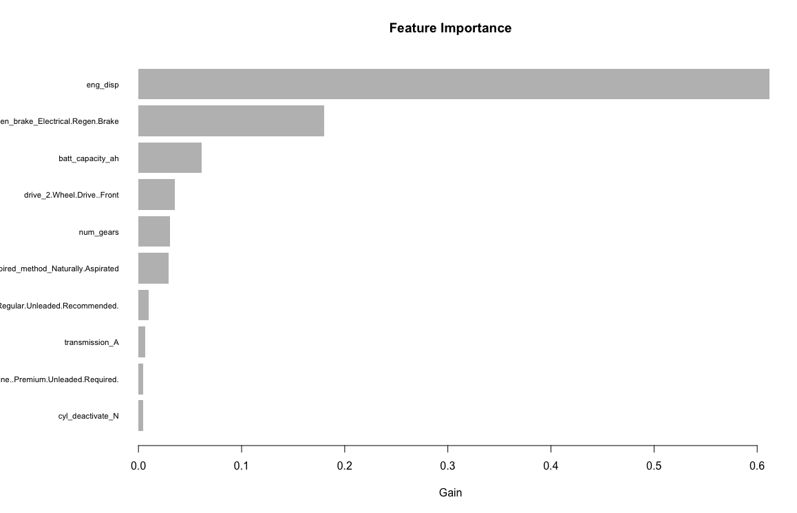
Similar to the other models, the variables/features I am using are: Engine displacement (size), number of cylinders, transmission type, number of gears, air inspired method, regenerative braking type, battery capacity Ah, drivetrain, fuel type, cylinder deactivate, and variable valve. Unlike the other models, the neuralnet package does not handle factors so I will have to transform them into dummy variables. After creating the dummy variables, I will be using 33 input variables.
The data which is all 2019 vehicles which are non pure electric (1253 vehicles) are summarized in previous posts below.
str(cars_19)
'data.frame':    1253 obs. of  12 variables:
 $ fuel_economy_combined: int  21 28 21 26 28 11 15 18 17 15 ...
 $ eng_disp             : num  3.5 1.8 4 2 2 8 6.2 6.2 6.2 6.2 ...
 $ num_cyl              : int  6 4 8 4 4 16 8 8 8 8 ...
 $ transmission         : Factor w/ 7 levels "A","AM","AMS",..: 3 2 6 3 6 3 6 6 6 5 ...
 $ num_gears            : int  9 6 8 7 8 7 8 8 8 7 ...
 $ air_aspired_method   : Factor w/ 5 levels "Naturally Aspirated",..: 4 4 4 4 4 4 3 1 3 3 ...
 $ regen_brake          : Factor w/ 3 levels "","Electrical Regen Brake",..: 2 1 1 1 1 1 1 1 1 1 ...
 $ batt_capacity_ah     : num  4.25 0 0 0 0 0 0 0 0 0 ...
 $ drive                : Factor w/ 5 levels "2-Wheel Drive, Front",..: 4 2 2 4 2 4 2 2 2 2 ...
 $ fuel_type            : Factor w/ 5 levels "Diesel, ultra low sulfur (15 ppm, maximum)",..: 4 3 3 5 3 4 4 4 4 4 ...
 $ cyl_deactivate       : Factor w/ 2 levels "N","Y": 1 1 1 1 1 2 1 2 2 1 ...
 $ variable_valve       : Factor w/ 2 levels "N","Y": 2 2 2 2 2 2 2 2 2 2 ...
First I need to normalize all the non-factor data and will use the min max method:
maxs <- apply(cars_19[, c(1:3, 5, 8)], 2, max)
mins <- apply(cars_19[, c(1:3, 5, 8)], 2, min)

scaled <- as.data.frame(scale(cars_19[, c(1:3, 5, 8)], center = mins, scale = maxs - mins))
tmp <- data.frame(scaled, cars_19[, c(4, 6, 7, 9:12)])
Neuralnet will not accept a formula like
fuel_economy_combined ~. so I need to write out the full model.
n <- names(cars_19)
f <- as.formula(paste("fuel_economy_combined ~", paste(n[!n %in% "fuel_economy_combined"], collapse = " + ")))
Next I need to transform all of the factor variables into binary dummy variables.
m <- model.matrix(f, data = tmp)
m <- as.matrix(data.frame(m, tmp[, 1]))
colnames(m)[28] <- "fuel_economy_combined")
I am going to use the geometric pyramid rule to determine the amount of hidden layers and neurons for each layer. The general rule of thumb is if the data is linearly separable, use one hidden layer and if it is non-linear use two hidden layers. I am going to use two hidden layers as I already know the non-linear svm produced the best model.
r = (INP_num/OUT_num)^(1/3)
HID1_num = OUT_num*(r^2)   #number of neurons in the first hidden layer
HID2_num = OUT_num*r          #number of neurons in the second hidden layer
This suggests I use two hidden layers with 9 neurons in the first layer and 3 neurons in the second layer. I originally fit the model with this combination but it turned out to overfit. As this is just a suggestion, I found that two hidden layers with 7 and 3 neurons respectively produced the best neural network that did not overfit.
Now I am going to fit a neural network:
set.seed(123)
indices <- sample(1:nrow(cars_19), size = 0.75 * nrow(cars_19))
train <- m[indices,]
test <- m[-indices,]

n <- colnames(m)[2:28]
f <- as.formula(paste("fuel_economy_combined ~", paste(n[!n %in% "fuel_economy_combined"], collapse = " + ")))
m1_nn <- neuralnet(f,
                   data = train,
                   hidden = c(7,3),
                   linear.output = TRUE)

pred_nn <- predict(m1_nn, test)

yhat <-pred_nn * (max(cars_19$fuel_economy_combined) - min(cars_19$fuel_economy_combined)) + min(cars_19$fuel_economy_combined)
y <- test[, 28] * (max(cars_19$fuel_economy_combined) - min(cars_19$fuel_economy_combined)) +min(cars_19$fuel_economy_combined)
postResample(yhat, y)
     RMSE  Rsquared       MAE
2.0036294 0.8688363 1.4894264
I am going to run a 20 fold cross validation to estimate error better as these results are dependent on sample and initialization of the neural network.
set.seed(123)
stats <- NULL

for (i in 1:20) {
  indices <- sample(1:nrow(cars_19), size = 0.75 * nrow(cars_19))
  train_tmp <- m[indices, ]
  test_tmp <- m[-indices, ]

  nn_tmp <- neuralnet(f,
                      data = train_tmp,
                      hidden = c(7, 3),
                      linear.output = TRUE)

  pred_nn_tmp <- predict(nn_tmp, test_tmp)

  yhat <- pred_nn_tmp * (max(cars_19$fuel_economy_combined) - min(cars_19$fuel_economy_combined)) + min(cars_19$fuel_economy_combined)
  y <- test_tmp[, 28] * (max(cars_19$fuel_economy_combined) - min(cars_19$fuel_economy_combined)) + min(cars_19$fuel_economy_combined)
  stats_tmp <- postResample(yhat, y)
  stats <- rbind(stats, stats_tmp)
  cat(i, "\n")
}
mean(stats[, 1] ^ 2)      #avg mse  4.261991
mean(stats[, 1] ^ 2) ^ .5 #avg rmse 2.064459

colMeans(stats) #ignore rmse
#RMSE Rsquared      MAE
#xxx  0.880502 1.466458
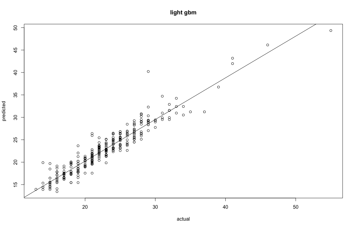
The neural network produces a RMSE of 2.06.
Comparison of RMSE:

svm = .93
gradient boosting = 1.8
random forest = 1.9
neural network = 2.06
decision tree = 2.49
mlr = 2.6