Data Science, Machine Learning and Predictive Analytics

R: MLR, Decision Trees and Random Forest to Predict MPG for 2019 Vehicles

I am going to use regression, decision trees, and the random forest algorithm to predict combined miles per gallon for all 2019 motor vehicles. The raw data is located on the EPA government site

After preliminary diagnostics, exploration and cleaning I am going to start with a multiple linear regression model.

The variables/features I am using for the models are: Engine displacement (size), number of cylinders, transmission type, number of gears, air inspired method, regenerative braking type, battery capacity Ah, drivetrain, fuel type, cylinder deactivate, and variable valve.

There are 1253 vehicles in the dataset (does not include pure electric vehicles) summarized below.

fuel_economy_combined    eng_disp        num_cyl       transmission
 Min.   :11.00         Min.   :1.000   Min.   : 3.000   A  :301     
 1st Qu.:19.00         1st Qu.:2.000   1st Qu.: 4.000   AM : 46     
 Median :23.00         Median :3.000   Median : 6.000   AMS: 87     
 Mean   :23.32         Mean   :3.063   Mean   : 5.533   CVT: 50     
 3rd Qu.:26.00         3rd Qu.:3.600   3rd Qu.: 6.000   M  :148     
 Max.   :58.00         Max.   :8.000   Max.   :16.000   SA :555     
                                                        SCV: 66     
   num_gears                      air_aspired_method
 Min.   : 1.000   Naturally Aspirated      :523     
 1st Qu.: 6.000   Other                    :  5     
 Median : 7.000   Supercharged             : 55     
 Mean   : 7.111   Turbocharged             :663     
 3rd Qu.: 8.000   Turbocharged+Supercharged:  7     
 Max.   :10.000                                     
                                                    
                 regen_brake   batt_capacity_ah 
             No        :1194   Min.   : 0.0000  
 Electrical Regen Brake:  57   1st Qu.: 0.0000  
 Hydraulic Regen Brake :   2   Median : 0.0000  
                               Mean   : 0.3618  
                               3rd Qu.: 0.0000  
                               Max.   :20.0000  
                                                
                     drive    cyl_deactivate
 2-Wheel Drive, Front   :345  Y: 172
 2-Wheel Drive, Rear    :345  N:1081
 4-Wheel Drive          :174  
 All Wheel Drive        :349  
 Part-time 4-Wheel Drive: 40  
                              
                              
                                      fuel_type   
 Diesel, ultra low sulfur (15 ppm, maximum): 28           
 Gasoline (Mid Grade Unleaded Recommended) : 16           
 Gasoline (Premium Unleaded Recommended)   :298                 
 Gasoline (Premium Unleaded Required)      :320                 
 Gasoline (Regular Unleaded Recommended)   :591                 
                                                                
                                                                
 variable_valve
 N:  38        
 Y:1215

Call:
lm(formula = fuel_economy_combined ~ eng_disp + transmission + 
    num_gears + air_aspired_method + regen_brake + batt_capacity_ah + 
    drive + fuel_type + cyl_deactivate + variable_valve, data = cars_19)

Residuals:
     Min       1Q   Median       3Q      Max 
-12.7880  -1.6012   0.1102   1.6116  17.3181 

Coefficients:
                                                   Estimate Std. Error t value Pr(>|t|)    
(Intercept)                                        36.05642    0.82585  43.660  < 2e-16 ***
eng_disp                                           -2.79257    0.08579 -32.550  < 2e-16 ***
transmissionAM                                      2.74053    0.44727   6.127 1.20e-09 ***
transmissionAMS                                     0.73943    0.34554   2.140 0.032560 *  
transmissionCVT                                     6.83932    0.62652  10.916  < 2e-16 ***
transmissionM                                       1.08359    0.31706   3.418 0.000652 ***
transmissionSA                                      0.63231    0.22435   2.818 0.004903 ** 
transmissionSCV                                     2.73768    0.40176   6.814 1.48e-11 ***
num_gears                                           0.21496    0.07389   2.909 0.003691 ** 
air_aspired_methodOther                            -2.70781    1.99491  -1.357 0.174916    
air_aspired_methodSupercharged                     -1.62171    0.42210  -3.842 0.000128 ***
air_aspired_methodTurbocharged                     -1.79047    0.22084  -8.107 1.24e-15 ***
air_aspired_methodTurbocharged+Supercharged        -1.68028    1.04031  -1.615 0.106532    
regen_brakeElectrical Regen Brake                  12.59523    0.90030  13.990  < 2e-16 ***
regen_brakeHydraulic Regen Brake                    6.69040    1.94379   3.442 0.000597 ***
batt_capacity_ah                                   -0.47689    0.11838  -4.028 5.96e-05 ***
drive2-Wheel Drive, Rear                           -2.54806    0.24756 -10.293  < 2e-16 ***
drive4-Wheel Drive                                 -3.14862    0.29649 -10.620  < 2e-16 ***
driveAll Wheel Drive                               -3.12875    0.22300 -14.030  < 2e-16 ***
drivePart-time 4-Wheel Drive                       -3.94765    0.46909  -8.415  < 2e-16 ***
fuel_typeGasoline (Mid Grade Unleaded Recommended) -5.54594    0.97450  -5.691 1.58e-08 ***
fuel_typeGasoline (Premium Unleaded Recommended)   -5.44412    0.70009  -7.776 1.57e-14 ***
fuel_typeGasoline (Premium Unleaded Required)      -6.01955    0.70542  -8.533  < 2e-16 ***
fuel_typeGasoline (Regular Unleaded Recommended)   -6.43743    0.68767  -9.361  < 2e-16 ***
cyl_deactivateY                                     0.52100    0.27109   1.922 0.054851 .  
variable_valveY                                     2.00533    0.59508   3.370 0.000775 ***
---
Signif. codes:  0 ‘***’ 0.001 ‘**’ 0.01 ‘*’ 0.05 ‘.’ 0.1 ‘ ’ 1

  standard error: 2.608 on 1227 degrees of freedom
Multiple R-squared:  0.8104,    Adjusted R-squared:  0.8066 
F-statistic: 209.8 on 25 and 1227 DF,  p-value: < 2.2e-16

The fitted MSE is 6.8 and predicted MSE of 6.83. Some of the below residuals are too large. The extreme large residual is a Hyundai Ioniq which none of the models predict very well as it is unique vehicle (versus the other data points).

Let's try a decision tree regression model.

#regression tree full
m_reg_tree_full <- rpart(formula = fuel_economy_combined ~ .,
                         data    = train,
                         method  = "anova",)
#regression tree tuned
m_reg_tree_trimmed <- rpart(
  formula = fuel_economy_combined ~ .,
  data    = train,
  method  = "anova",
  control = list(minsplit = 10, cp = .0005)
)

#rpart.plot(m_reg_tree_full)
plotcp(m_reg_tree_full)

pred_decision_tree_full <- predict(m_reg_tree_full, newdata = test)
mse_tree_full <- RMSE(pred = pred_decision_tree_full, obs = test$fuel_economy_combined) ^2

pred_decision_tree_trimmed <- predict(m_reg_tree_trimmed, newdata = test)
mse_tree_trimmed <- RMSE(pred = pred_decision_tree_trimmed, obs = test$fuel_economy_combined) ^2
plotcp(m_reg_tree_trimmed)

After tuning the decision tree the predicted MSE is 6.20 which is better than the regression model.

Finally let's try a random forest model. The random forest should produce the best model as it will attempt to remove some of the correlation within the decision tree structure.

#random forest
m_random_forest_full <-randomForest(formula = fuel_economy_combined ~ ., data = train)
predict_random_forest_full <- predict(m_random_forest_full, newdata = test)
mse_random_forest_full <- RMSE(pred = predict_random_forest_full, obs = test$fuel_economy_combined) ^ 2

which.min(m_random_forest_full$mse)

#random forest tuned
m_random_forest <- randomForest(formula = fuel_economy_combined ~ ., data = train, ntree = 250)
plot(m_random_forest)
predict_random_forest <- predict(m_random_forest, newdata = test)
mse_random_forest <- RMSE(pred = predict_random_forest, obs = test$fuel_economy_combined) ^ 2

plot(tmp$test.fuel_economy_combined - tmp$r.predict_random_forrest., ylab = "residuals",main = "Random Forest")

varImpPlot(m_random_forest)

The error stabilizes at 250 trees. randomForest() by default uses 500 trees which is unnecessary.

After tuning the random forest the model has the lowest fitted and predicted MSE of 3.67 which is substantially better than the MSE of the decision tree 6.2

The random forest also has an r-squared of .9

Engine size, number of cylinders, and transmission type are the largest contributors to accuracy.

R: K-Means Clustering MLB Data

k-means clustering is a useful unsupervised learning data mining tool for assigning n observations into k groups which allows a practitioner to segment a dataset.

I play in a fantasy baseball league and using five offensive variables (R, AVG, HR, RBI, SB) I am going to use k-means clustering to:

1) Determine how many coherent groups there are in major league baseball. For example,

is there a power and high average group? Is there a low power, high average, and speed group?

2) Assign players to these groups to determine which players are similar or can act as replacements. I am not using this algorithm to predict how players will perform in 2017.

For a data source I am going to use all MLB offensive players in 2016 which had at least 400 plate appearances from baseball-reference This dataset has n= 256 players.

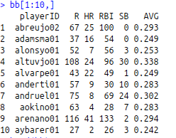
Sample data below

Step 1

How many k groups should I use?

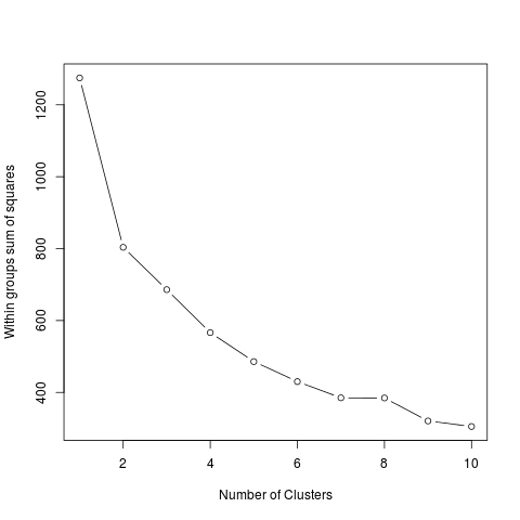
The within groups sum of squares plot below suggests k=7 groups is ideal. k=9 is too many groups for n=256 and the silhouette plot for k=9 is poor.

Step 2

Is k=7 groups a good solution?

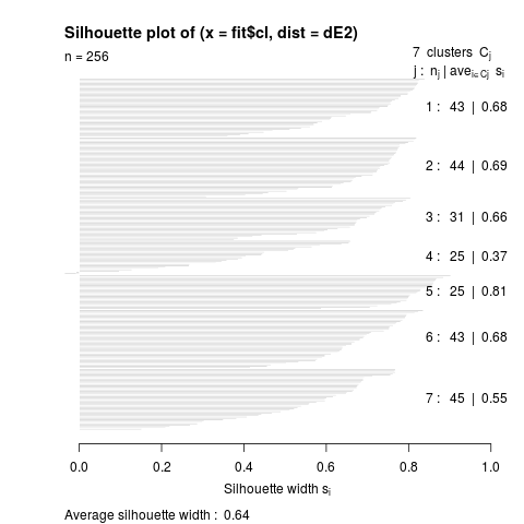
Let's look at a silhouette plot to look at the fit of each cluster and the overall k=7 clusters.

The average silhouette width = .64 indicates a reasonable structure has been found. Cluster 4 which is the speed group has a low silhouette width of .37. I am OK with this as it is the smallest group and speed is the hardest offensive tool to find in MLB.

Step 3

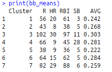
Calculate group means for k=7 groups

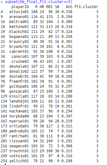
Players that are classified in cluster 3 are the elite players in MLB. Based on 2016 stats, 31 players make up cluster 3. On average they have the highest AVG, R, RBI, HR, and the second highest SB.

Adding Hampel Psi Function to robustreg

I am currently working on adding the Hampel psi function to robustreg.

Pure R implementation:

psiHampel <- function(r, a, b, c) {
    psi <- NULL
    for (i in 1:length(r)) {
        if (abs(r[i]) <= a) {
            psi[i] <- r[i]
        } else if (abs(r[i]) > a & abs(r[i]) <= b) {
            psi[i] <- a * sign(r[i])
        } else if (abs(r[i]) > b & abs(r[i]) <= c) {
            psi[i] <- (a * (c - abs(r[i]))/(c - b)) * sign(r[i])
        } else {
            psi[i] <- 0
        }
    }
    return(psi)
}

Rcpp/C++ implementation:

#include <Rcpp.h>
#include <math.h>
using namespace Rcpp;
using namespace std;

// [[Rcpp::export]]
NumericVector psiHampel_rcpp(NumericVector r, double a, double b, double c)
{
    int n = r.size();
    NumericVector y = clone(r);

    for (int i = 0; i < n; i++) {
        if (abs(r[i]) <= a) {
            y[i] = r[i];
        }
        else if (
            abs(r[i]) > a && abs(r[i]) <= b) {
            if (r[i] > 0) {
                y[i] = a;
            }
            else {
                y[i] = -a;
            }
        }
        else if (
            abs(r[i]) > b && abs(r[i]) <= c) {
            if (r[i] > 0) {
                y[i] = (a * (c - abs(r[i])) / (c - b));
            }
            else {
                y[i] = (a * (c - abs(r[i])) / (c - b) * -1);
            }
        }
        else {
            y[i] = 0;
        }
    }
    return y;
}

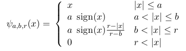
Below is a ggplot2 graph of values a=2, b=4, c=8 where x ranges from -10 to 10:

z=seq(-50,50,.01) all.equal(psiHampel(z,2,4,8), psiHampel_rcpp(z,2,4,8)) [1] TRUE

Both functions have the same result although the C++ implementation is much faster.

R: Baseball Pitching Wins Above Replacement and Salary

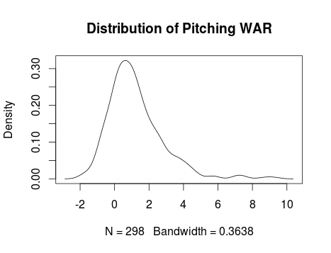
Are elite baseball pitchers worth their salaries? To investigate this I fitted linear and robust linear models using Baseball-Reference.com definition of wins above replacement. The universe of data is all pitchers in the year 2015 who started at least 20 games or as a reliever pitched 70 outs which is 298 players.

The distribution of war is below:

Min. 1st Qu. Median Mean 3rd Qu. Max.
-1.79 0.2125 0.95 1.219 1.905 9.28

standard dev: 1.61
mad: 1.245

Fitting a linear model to the data:

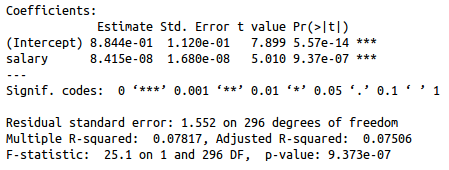
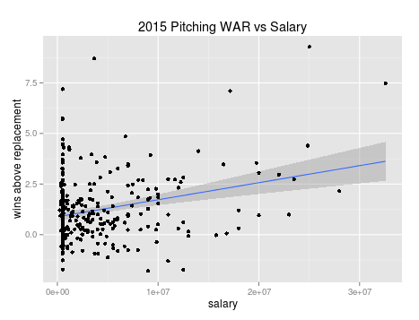
We can see that there is a linear relationship between salary and war as salary is significant. The correlation between the two variables is ~.28 but the MSE is 2.4 which indicates the model isn't the best fit. The linear model suggests that each additional $11,883,599 in player salary should buy a win over a replacement player.

Investigating a robust model:

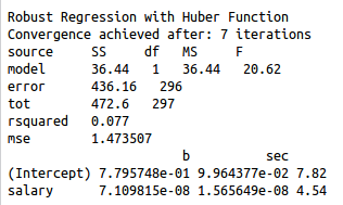
The robust model is a better fit as MSE is significantly lower at 1.47. The correlation between salary and war is slightly lower at .277. The advantage of a robust model is it will minimize outliers by assigning lower weights. The robust model suggests that each additional $14,065,063 in player salary should buy a win over a replacement player.

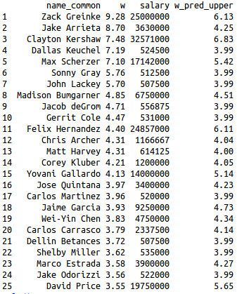
Below is a table of 2015 war, 2015 salary, and the upper prediction interval of war based on 2015 salary:

The top ten pitchers in 2015 all had better seasons than the upper end of the prediction interval based on their salary.

R Text Mining: The Wells Report

Word Cloud Wells Report

Story: Patriots Deflated Footballs
Document to be text mined: Wells Report

How to Create Word Cloud using R:

Packages needed:
tm: Text Mining Package
RColorBrewer: ColorBrewer Palettes
wordcloud: Word Clouds

1) Convert PDF to text file using pdftotext

2) Clean the document and remove numbers, punctuation, symbols, and stop words.

 library(tm) #text mining   
 source<-DirSource("~/Text") #save text file(s) here   
 a<-Corpus(source, readerControl=list(reader=readPlain))   
 a <- tm_map(a, content_transformer(removeNumbers))   
 a <- tm_map(a, content_transformer(removePunctuation))   
 a <- tm_map(a, content_transformer(tolower))   
 a<- tm_map(a, stripWhitespace)   
 a[[1]] <- removeWords(a[[1]], stopwords("en"))   
 a<- tm_map(a, stripWhitespace)

3) Examine the corpus and replace words if necessary. Since the Wells report was written by two parties, a lawfirm and Exponent some of the terms were inconsistent. This is how I changed "psig" to "psi" which were used interchangeably in the document:

 a[[1]]<- gsub( "psig" , "psi" , a[[1]])   
 a<- tm_map(a, PlainTextDocument) #neccessary after word replacement

4) Create term document matrix and dataframe of keywords:

 tdm<- TermDocumentMatrix(a, control = list(minWordLength = 3))   
 keywords<-tdm[[6]][[1]]   
 count<-tdm[[3]]   
 k<-data.frame(keywords,count)   
 k<-k[order(-k[,2]),]

5) Create and format word cloud:

 library(RColorBrewer) #colors wordcloud   
 library(wordcloud)   
 tdm.m <- as.matrix(tdm)   
 tdm.v <- sort(rowSums(tdm.m),decreasing=TRUE)   
 tdm.d <- data.frame(word = names(tdm.v),freq=tdm.v)   
 table(tdm.d$freq)   
 pal2 <- brewer.pal(8,"Dark2")   
 png("wells_report.png", width=8,height=8, units='in', res=400)   
 wordcloud(tdm.d$word,tdm.d$freq, scale=c(8,.2),min.freq=5, max.words=Inf,  random.order=FALSE, rot.per=.15, colors=pal2)   
 dev.off()

Three Card Poker Game for R

A few years ago I created a comprehensive simulation of the card game three card poker for a client in Las Vegas. I recently converted the simulation into a simple command line game for R.

Three Card Poker Game for R (Linux)
Three Card Poker Game for R (Windows)

UPDATED 7/16/2015

Benefits and Uses of Statistical Research

Identify Risk or Opportunity
Statistical research and data mining models can be used to identify both specific risk or opportunity to a company. Credit card companies use data mining models to identify possible fraudulent transactions or the probability of a consumer to default on a loan or miss a payment. Statistical research can also be used to identify high quality consumers that will minimize possible borrowing risks and maximize earnings.

Market Segmentation
Statistical research can be used to identify high quality consumers who are profitable to retain and low quality consumers who are not profitable to retain. High quality consumers who are at risk of canceling a service might respond to a particular marketing strategy with a higher probability rather than an alternative strategy. Statistical research and predictive modeling techniques can be used to maximize the retention of quality consumers.

Cross Selling
Companies today collect vast data concerning their customers including demographics and purchasing habits and behavior. Statistical research and data mining models can be used to identify current consumers that are likely to purchase additional products from organizations that maintain and collect elaborate data.

Identify New Markets
Statistical research can be used to identify new markets and opportunities. A properly designed survey and sampling techniques can be used to identify consumers that are likely to purchase a brand new product and whether it would be profitable for a company to bring it to market.

Minimize Variability of a Process
Many times a company may be more concerned about the variability of a response around its mean rather than the actual mean response. Statistical research can be used to ensure homogeneity of product rather than products that are manufactured with different tolerance levels. As an example, a company manufacturing semiconductors that need to fit into another company's motherboard would want to minimize variability in dimensions and thickness to ensure the products fit and are compatible rather than focus on the mean of product dimensions.

Efficacy of a Process or Product using Design of Experiments
Proper experimental design including randomization, replication, and blocking (if necessary) can determine if a drug, diet, exercise program, etc. is effective versus another. Choosing the correct design before the experiment and appropriate factors and interactions to investigate is critical. Types of designs include completely randomized designs (CRD), CRD with blocking, split plot designs, full and partial factorial designs, etc.